
Do You Know the Finite Element Method?
Published:
Introduction
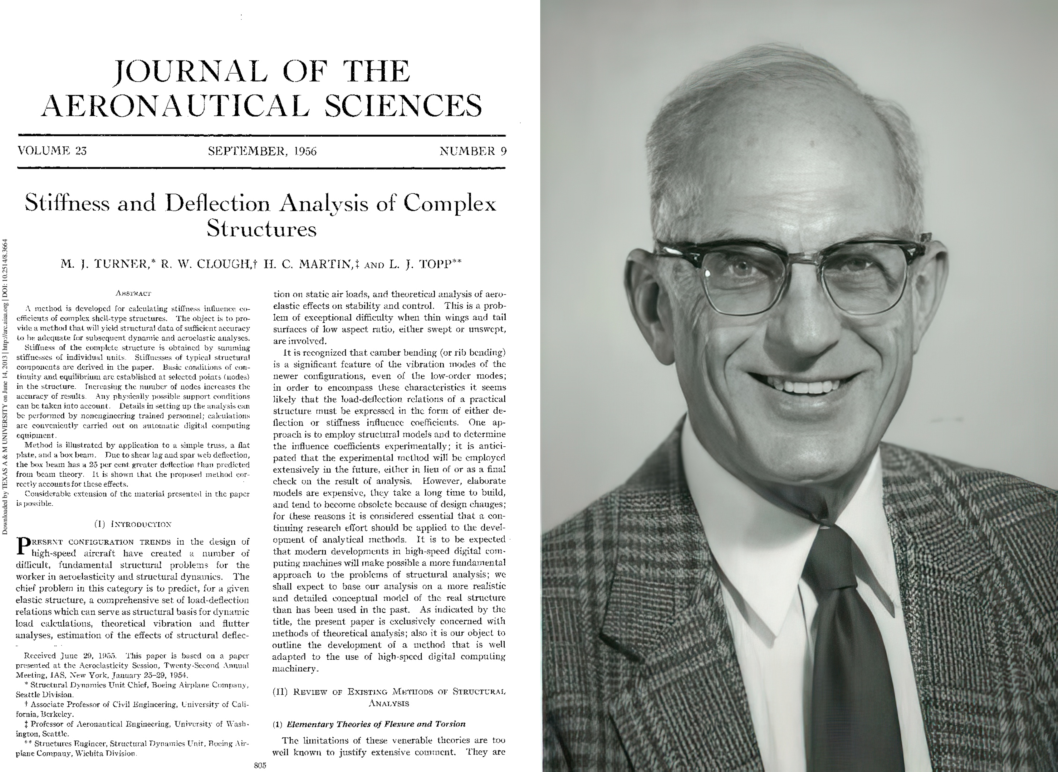
Fig. 1. Left: Cover of the paper 'Stiffness and Deflection Analysis of Complex Structures' published in the Journal Of The Aeronautical Sciences. Right: Photograph of civil engineer Ray William Clough, one of the founders of FEM.
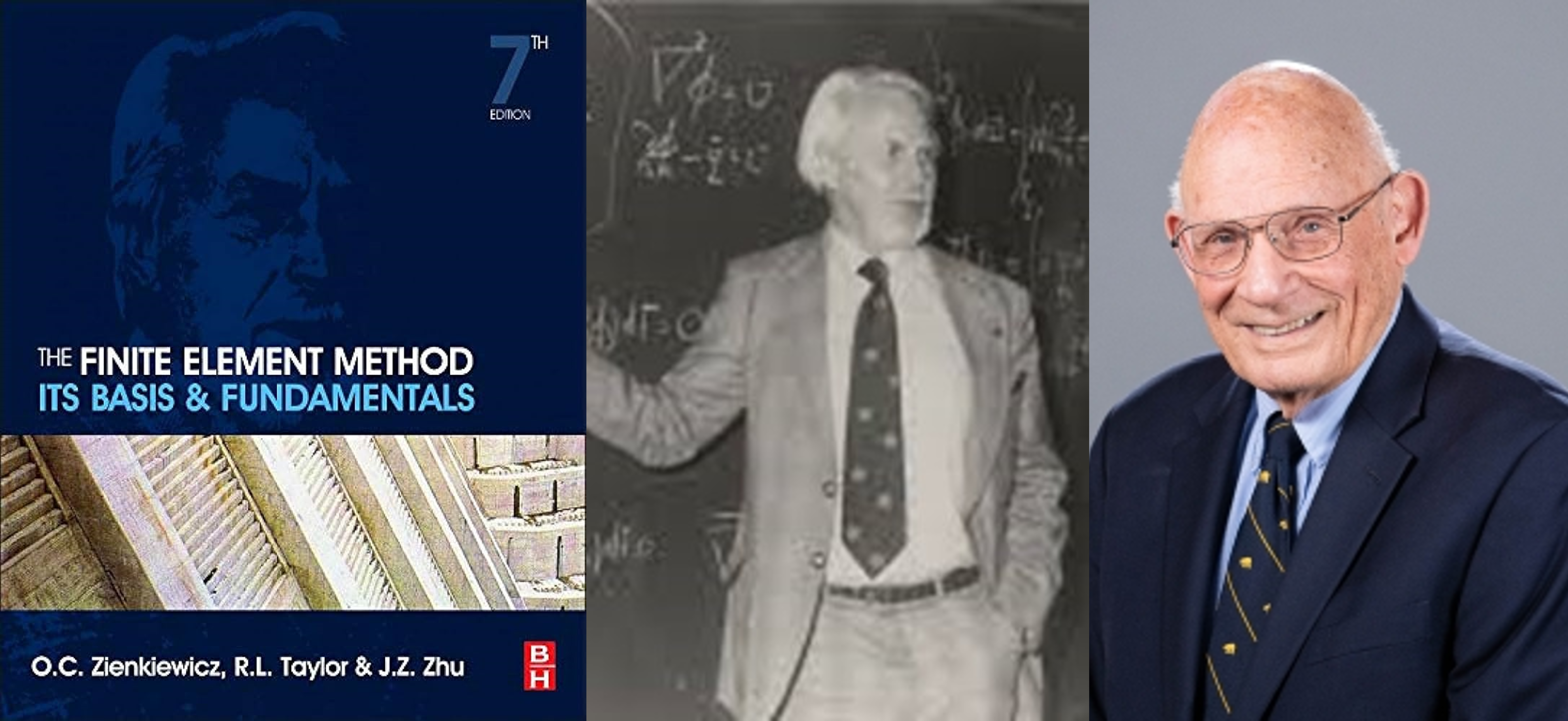
Fig. 2. Left to right: Cover of the book 'The Finite Element Method.' Photograph of civil engineer Olgierd Zienkiewicz followed by civil engineer Robert L. Taylor.
Basic Concepts of FEM
- Domain Discretization: Discretization is the process of dividing the continuous domain of a problem into a mesh of finite elements. This mesh can be structured (with regularly shaped elements) or unstructured (with irregularly shaped elements), depending on the geometry of the domain and the nature of the problem. For example, in the analysis of a beam, the beam can be divided into a series of smaller segments (elements) connected at points (nodes). Each node can have one or more degrees of freedom, such as vertical displacements and rotations.
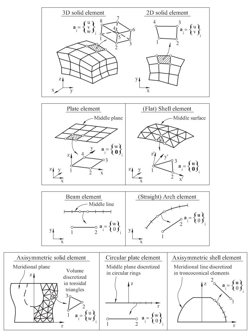
Fig. 3. Discretization of structural models into finite elements. Taken from '(Oñate, E. 2009)'.
Formulation of Elemental Equations: For each finite element, equations describing its behavior are derived using physical and mathematical principles. These equations are usually expressed in terms of a stiffness matrix (for structural problems) or a thermal conductivity matrix (for heat transfer problems). The typical formulation involves using shape functions, which are mathematical functions that interpolate the problem variables’ values between the element’s nodes. These functions allow the solution to be approximated within each element based on the nodal values.
Assembly of the Global System of Equations: The elemental equations are assembled into a global system of equations representing the behavior of the entire discretized domain. This assembly is done by summing the contributions of all elements that share common nodes. The result is a system of linear equations of the form: 𝐊𝐮 = 𝐟, where 𝐊 is the global stiffness matrix, 𝐮 is the vector of unknown nodal displacements, and 𝐟 is the vector of applied nodal forces.
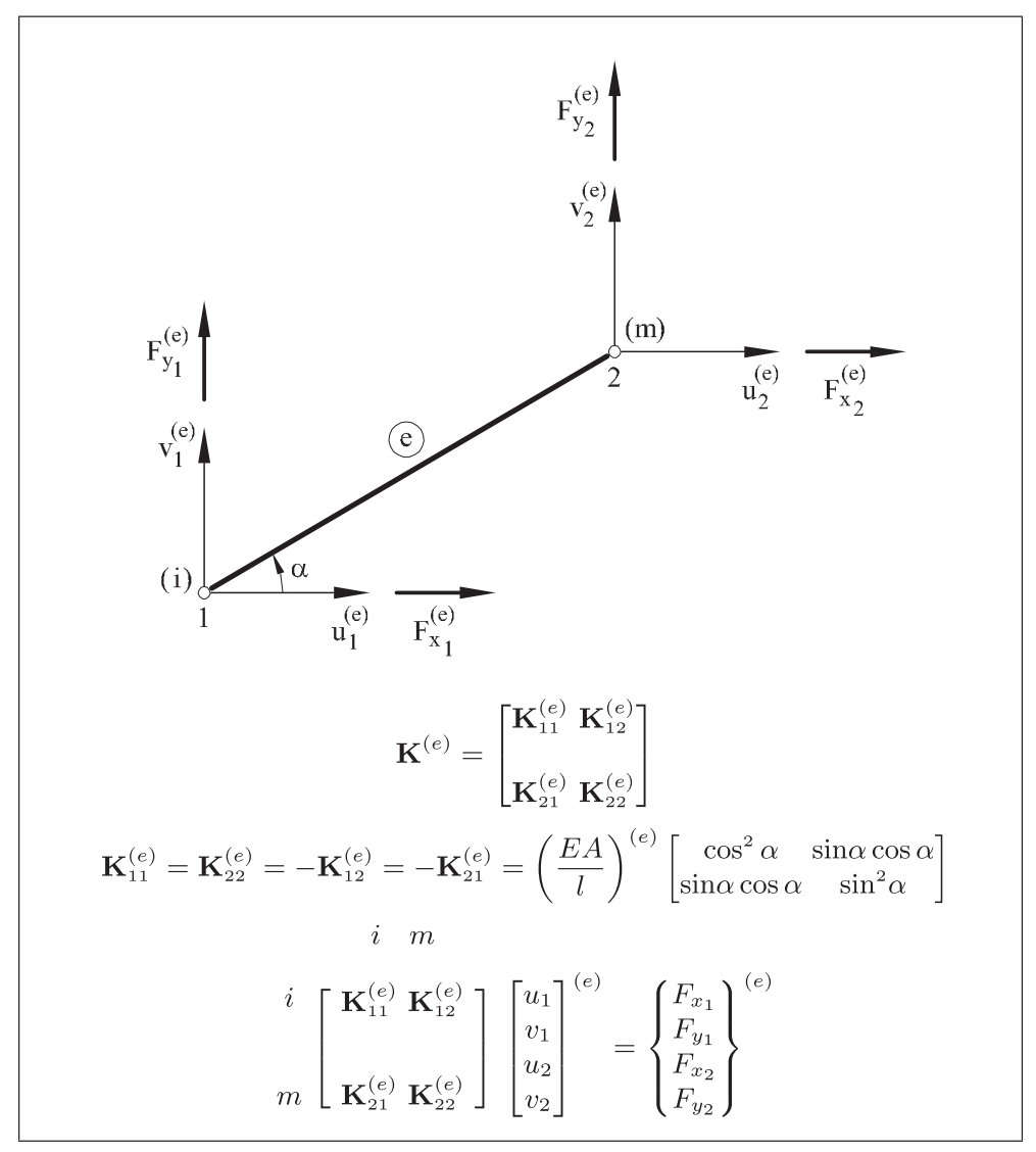
Fig. 4. Contributions to the global stiffness matrix. Taken from '(Oñate, E. 2009)'.
Application of Boundary Conditions: Boundary conditions specify the values of the problem variables at the domain’s boundaries. These conditions can be of Dirichlet type (fixed values of the variables) or Neumann type (fixed values of the derivatives of the variables). In the case of the beam, we could have boundary conditions that specify that the beam’s ends are fixed (zero displacements and rotations) or that a specific force acts at a point on the beam.
Solving the System of Equations: The global system of equations is solved using numerical methods to obtain the problem variables at the nodes. The most common methods include Gaussian elimination, LU decomposition, and iterative methods such as the Jacobi method or the Gauss-Seidel method.
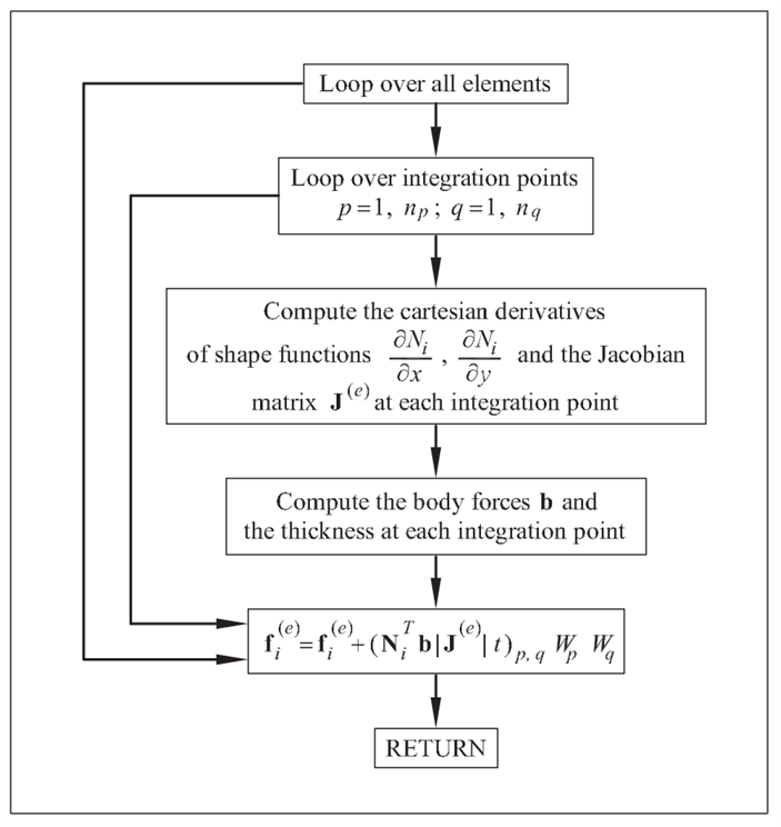
Fig. 5. Flowchart for calculating f(e) for body forces. Taken from '(Oñate, E. 2009)'.
- Post-Processing of Results: Once the system is solved, the results are interpreted to evaluate the variables of interest. This can include visualizing displacements, stresses, temperatures, etc., using graphical post-processing tools.
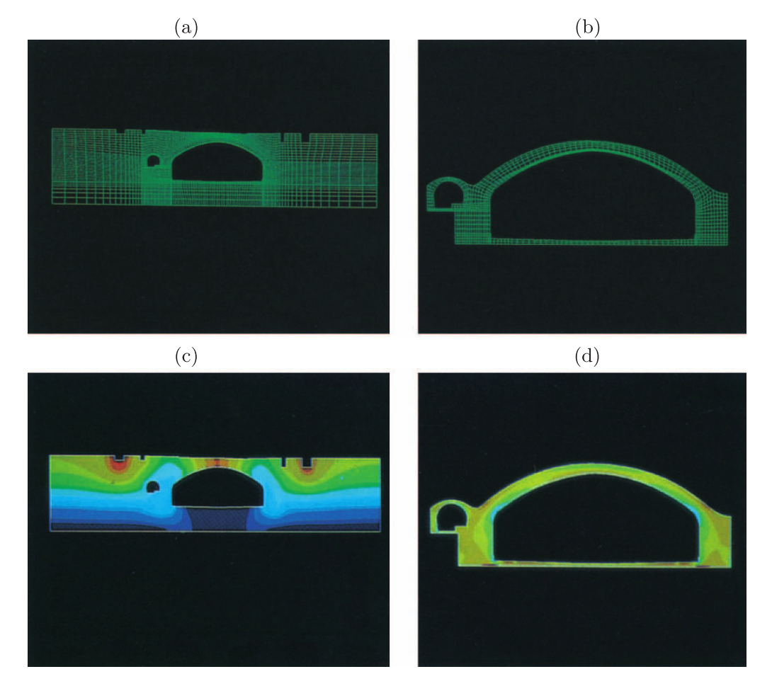
Fig. 6. Underground tunnel. a) Serendipity quadrilateral mesh with 8 nodes, b) Mesh detail, c) Total displacement contours for self-weight load plus adjacent buildings' weight, d) Detail of minor principal stress contours. Taken from '(Oñate, E. 2009)'.
Applications of FEM
- Structural Analysis: Structural analysis represents one of the most widespread applications of FEM. This method is employed to determine the response of structures subjected to various loads and conditions. In the construction sector, FEM is used to analyze the distribution of stresses and deformations in building and bridge structures, considering dead loads, live loads, wind loads, and earthquakes. This facilitates the evaluation of the strength and stability of structures, allowing the identification of possible critical points and optimizing their design. In the aerospace industry, it is crucial for analyzing wings, fuselages, and other aircraft components, ensuring their capacity to withstand aerodynamic loads during flight and landing, as well as evaluating aspects like material fatigue and vibrations. In automotive and heavy machinery engineering, FEM is used to examine chassis, suspensions, and structural components, ensuring they meet strength and durability requirements under various operating conditions.
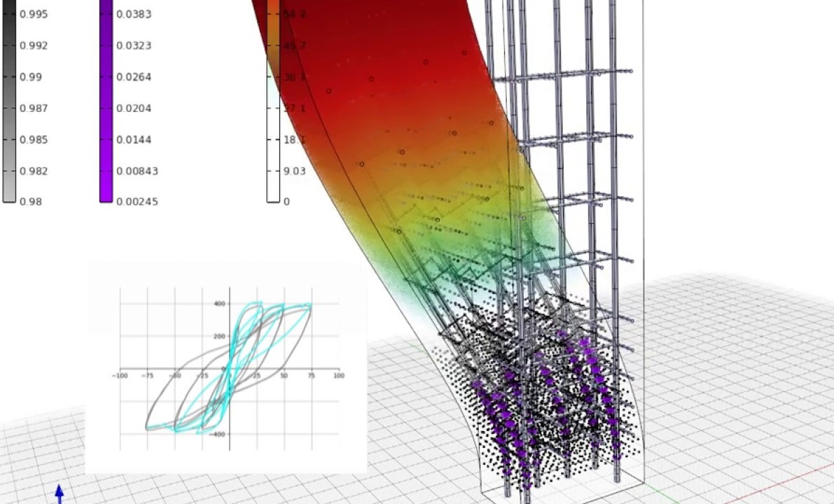
Fig. 7. Detailed 3D macromodeling of a reinforced concrete column using finite elements. Taken from 'Asdea Software Technology'.
- Heat Transfer: FEM is a vital tool for solving heat transfer problems in solids and fluids. For example, in the design of heat exchangers, it allows for analyzing temperature distribution and thermal gradients, optimizing design to improve thermal efficiency and minimize energy losses. In the metallurgical industry, it is used to simulate casting and welding processes, predicting temperature distribution and thermal stresses that may generate material defects. Additionally, it is applied in the design and analysis of cooling and heating systems, ensuring uniform temperature distribution and energy efficiency of the system.
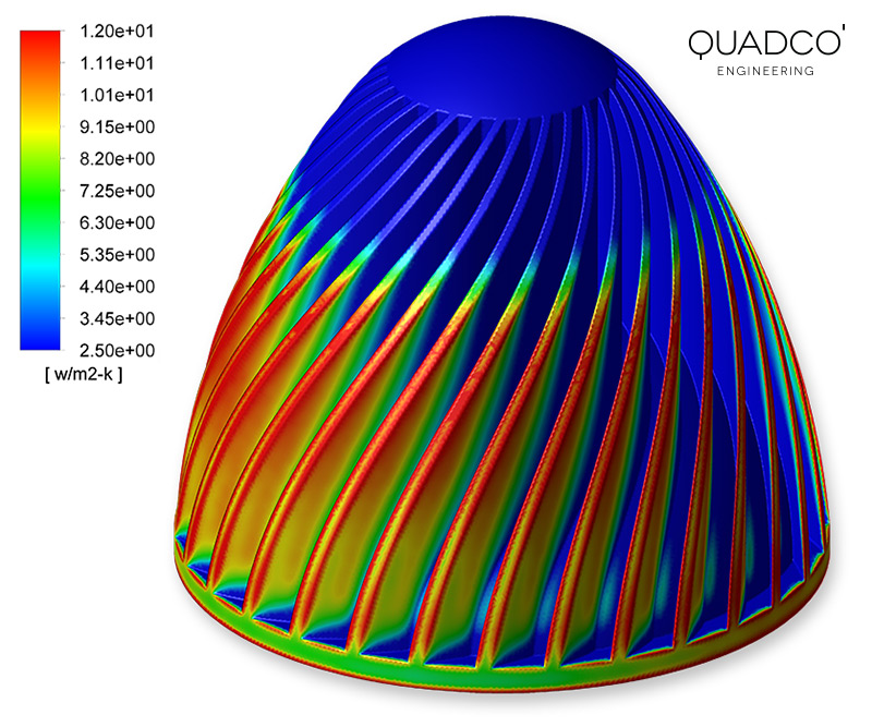
Fig. 8. Temperature varying with time in an LED heat sink during heating. Taken from 'Quadco Engineering'.
- Fluid Dynamics (Computational Fluid Dynamics: “CFD”): CFD greatly benefits from FEM, enabling the analysis of complex flows in various applications. In the aeronautical and automotive sectors, it is used to simulate airflows around aircraft and vehicles, evaluating aerodynamics, drag, and behavior under different flight or driving conditions. In hydraulic engineering, it is applied to analyze water flow in channels, pipes, and dams. It is also used in the energy sector to simulate flow in turbines and wind and marine energy systems. Furthermore, it allows for simulating fluid flow in industrial processes, such as liquid mixing in chemical reactors, gas flow in ventilation systems, and fluid distribution in complex piping systems.
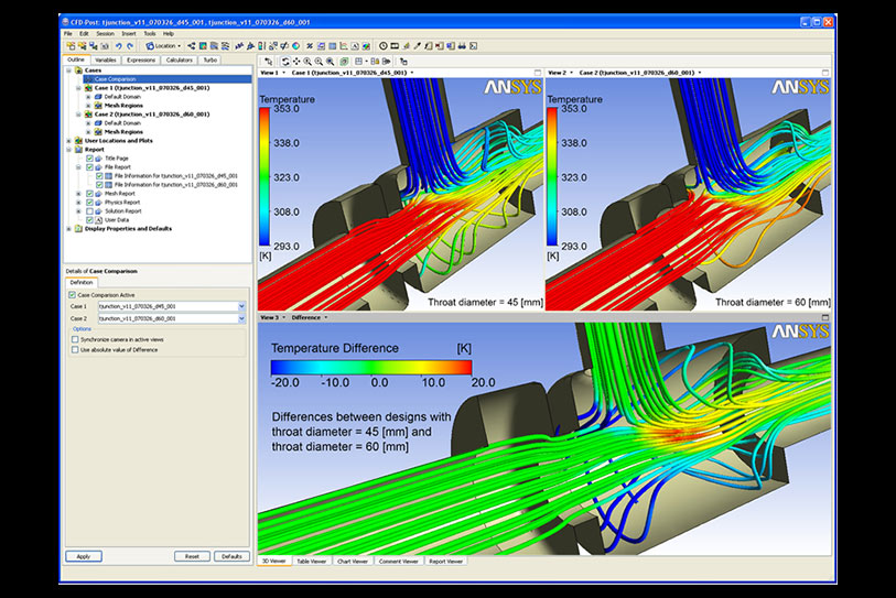
Fig. 9. Computational fluid dynamics analysis. Taken from 'Solenoid Systems'.
- Electromagnetism: FEM is also applied in the analysis of electromagnetic fields for various applications. It is used to analyze the electromagnetic behavior of electronic devices, such as antennas, sensors, and printed circuits, optimizing their design to improve efficiency and minimize interference. In electrical engineering, it allows for modeling and analyzing the distribution of electric and magnetic fields in power generation, transmission, and distribution systems, ensuring the safe and efficient operation of equipment. Additionally, it helps evaluate and mitigate electromagnetic compatibility issues in electronic devices and systems, reducing interference and improving product reliability.
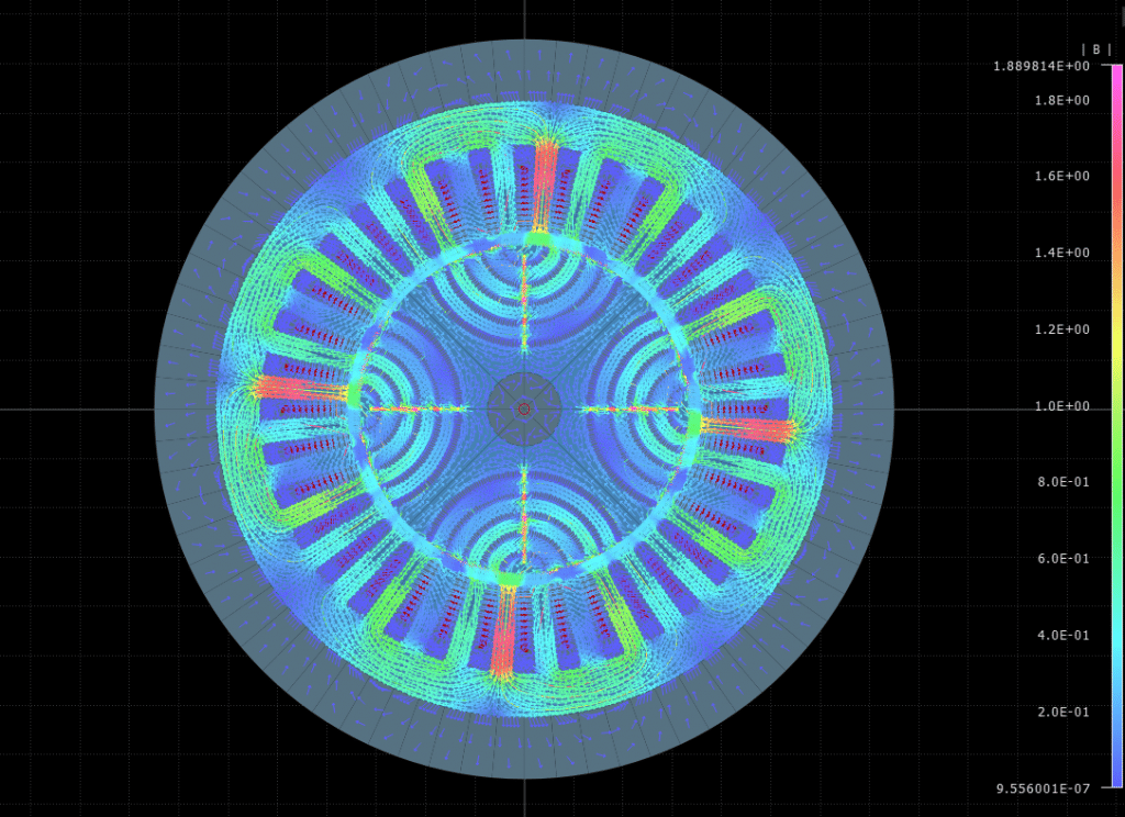
Fig. 10. Finite element simulation of the electromagnetic field for automobiles. Taken from 'Entekmograte'.
- Biomechanics: In the field of biomechanics, FEM is used to study the behavior of tissues and biological structures. It allows for the design and optimization of prostheses and orthoses by analyzing the distribution of stresses and deformations in the material and at the contact points with the human body, improving comfort and functionality. It is also applied in the design of orthopedic and dental implants, ensuring that the materials and geometries used are compatible with the biomechanical conditions of the human body. Furthermore, it is used to study the mechanics of biological tissues, such as bones, muscles, and arteries, facilitating the understanding of injuries and the development of more effective treatments.
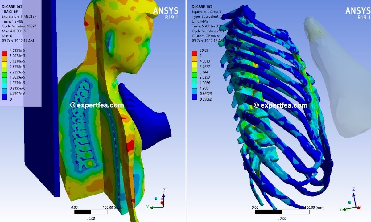
Fig. 11. Biomechanical simulation of a chest kick. Taken from 'ANSYS'.
Advantages of FEM
Geometric Flexibility: FEM is notable for its ability to model domains with arbitrary and complex geometries, which is highly useful in engineering and architecture where structures may have irregular and complex shapes. The finite element mesh is highly adaptable and can be easily adjusted to accommodate changes in the model’s design. This flexibility is fundamental in iterative design and optimization processes, allowing for continuous modifications without compromising the integrity of the analyzed model.
Adaptability and Refinement: One of the most prominent features of FEM is its ability to refine the mesh in specific areas of the domain that require greater attention, such as zones where stresses are concentrated or where significant thermal gradients exist. This improves result accuracy without unnecessarily increasing computational cost for the entire domain. The ability to vary the size and shape of elements within the same mesh adds an additional layer of flexibility and efficiency in representing the studied domain.
Versatility in Applications: FEM is applicable to a vast range of problems across various areas, such as structural mechanics, heat transfer, fluid dynamics, electromagnetism, and acoustics. This versatility makes it especially valuable for addressing nonlinear problems, including large deformations, plasticity, contact between surfaces, and fractures. These characteristics are essential for the detailed analysis of materials and structures subjected to extreme and challenging conditions.
Precision and Convergence: The precision of FEM can be effectively controlled through mesh refinement and the selection of appropriate interpolation functions for the elements used. This methodological approach ensures that the solution converges to the exact value as the mesh is refined, provided that suitable elements are used and best modeling practices are followed. This ensures reliable and accurate results, which are fundamental for decision-making in engineering design and analysis.
Limitations of FEM
Computational Requirements: Analysis using FEM can be intensive in terms of memory and processing time, especially when handling large and complex models. This demand may require the use of supercomputers or high-performance clusters to adequately manage the computational loads and data storage.
Dependence on Mesh Quality: The quality of the mesh has a significant impact on the accuracy and stability of the results obtained using FEM. An inadequately defined mesh can result in inaccurate results or even non-convergence of the model. Developing suitable meshes for complex geometries is a process that can be complicated and laborious, requiring significant experience and the use of advanced software tools.
Experience and Knowledge Required: Effective implementation of FEM requires a high level of knowledge and experience. This includes a solid understanding of the underlying physical, mathematical, and numerical principles. Additionally, the correct choice of constitutive models, material parameters, and interpolation functions is critical, as they can significantly affect the quality of results. This necessity underscores the importance of having expert judgment and deep knowledge of the specific problem to be solved.
Specific Problems and Intrinsic Limitations: In applications such as structural dynamics and high-frequency acoustics, FEM may require excessive mesh refinement, increasing the computational cost of the analysis. Additionally, FEM may face difficulties in multiscale problems, where relevant phenomena manifest on multiple time and length scales. In these cases, it may be necessary to integrate FEM with other numerical methods to achieve precise and reliable results.
Conclusions
Bibliography
- Belytschko, T., Liu, W. K., Moran, B., & Elkhodary, K. (2014). Nonlinear finite elements for continua and structures. John Wiley & Sons.
- Clough, R. W. (1990). Original formulation of the finite element method. Finite Elements in Analysis and Design, 7(2), 89-101.
- Courant, R. (1994). Variational methods for the solution of problems of equilibrium and vibrations. Lecture Notes in Pure and Applied Mathematics, 1-1.
- Hughes, T. J. (2003). The finite element method: linear static and dynamic finite element analysis. Courier Corporation.
- Oñate, E. (2009). Introduction to the finite element method for structural analysis. Structural Analysis with the Finite Element Method: Linear Statics, 1-42.
- Reddy, J. N. (2019). Introduction to the finite element method. McGraw-Hill Education.
- Turner, M. J., Clough, R. W., Martin, H. C., & Topp, L. J. (1956). Stiffness and deflection analysis of complex structures. Journal of the Aeronautical Sciences, 23(9), 805-823.
- Zienkiewicz, O. C., & Taylor, R. L. (2005). The finite element method set. Elsevier.